2022-10-21发表2022-10-21更新 yalechen 2 分钟读完 (大约278个字)

前端框架检查规则包

腾讯云代码分析 TCA - 前端框架检查规则包

背景

前端项目在长期发展过程中，由于框架开源许可证变更、框架性能外观等不适用等因素，需要对前端框架进行平滑切换，而这就需要腾讯云代码分析 TCA 的介入，方便对企业内所有前端项目进行批量分析统计，方便管理。

需求

检查代码仓库中使用到指定前端框架的代码位置。

示例

{
  "name": "framework",
  "version": "1.0.0",
  "dependencies": {
    "react": "^17.0.2", // 触发规则
    "react-dom": "^17.0.2", // 触发规则
    "react-hotkeys-hook": "^3.4.3", // 触发规则
    "react-redux": "^7.2.5", // 触发规则
    "single-spa": "^5.9.3",
    "universal-cookie": "^4.0.4"
  },
}

快速体验

TCA 现已支持前端框架检查规则包，可以在 TCA 分析方案中搜索勾选以下规则包，快速体验。

启用规则包

分析方案 -> 代码检查 -> 前端框架检查规则包 -> 启用/查看规则

支持框架

TDesign
AntD
React
Vue

更多框架支持，欢迎提 issue 进行咨询扩展。

2022-07-30发表2022-07-30更新 yalechen 35 分钟读完 (大约5294个字)

2022-7-30-Binaryen-Readme

Binaryen

Binaryen 是一个用于 WebAssembly 的编译器和工具链基础设施库，用 C++ 编写。它旨在使编译成 WebAssembly 简单、快速和高效:

简单: Binaryen 提供了个简单的 C API，也可以
使用 JavaScript 调用. 它接受来自类 WebAssembly
格式的输入，也接受一个通用的 control flow graph.
快速: Binaryen 的内部 IR 使用紧凑的数据结构，专为完全并行的代码生成和优化而设计，使用所有可用的 CPU 内核。 Binaryen 的 IR 也非常容易和快速地编译成 WebAssembly，因为它本质上是 WebAssembly 的一个子集。
高效:
Binaryen 的优化器有许多可以改进代码大小和速度的关卡pass（参见后面的概述）。这些优化旨在使 Binaryen 足够强大，可以单独用作编译器后端。一个特定的关注领域是特定于 WebAssembly 的优化（通用编译器可能不会这样做），您可以将其视为 wasm minification，类似于 JavaScript、CSS 等的缩小版，所有这些都是具体的语言。

Compilers using Binaryen include:

AssemblyScript 它将 TypeScript 的变体编译为 WebAssembly
wasm2js 支持将 WebAssembly 编译成 JS
Asterius which compiles Haskell to WebAssembly
Grain which compiles Grain to WebAssembly

Binaryen also provides a set of toolchain utilities that can

Parse and emit WebAssembly. In particular this lets you load
WebAssembly, optimize it using Binaryen, and re-emit it, thus implementing a
wasm-to-wasm optimizer in a single command.
Interpret WebAssembly as well as run the WebAssembly spec tests.
Integrate with Emscripten in order to provide a
complete compiler toolchain from C and C++ to WebAssembly.
Polyfill WebAssembly by running it in the interpreter compiled to
JavaScript, if the browser does not yet have native support (useful for
testing).

Consult the contributing instructions if you’re interested in
participating.

Binaryen IR

Binaryen’s internal IR is designed to be

Flexible and fast for optimization.
As close as possible to WebAssembly so it is simple and fast to convert
it to and from WebAssembly.

There are a few differences between Binaryen IR and the WebAssembly language:

Tree structure
- Binaryen IR is a tree, i.e., it has hierarchical structure,
  for convenience of optimization. This differs from the WebAssembly binary
  format which is a stack machine.
- Consequently Binaryen’s text format allows only s-expressions.
  WebAssembly’s official text format is primarily a linear instruction list
  (with s-expression extensions). Binaryen can’t read the linear style, but
  it can read a wasm text file if it contains only s-expressions.
- Binaryen uses Stack IR to optimize “stacky” code (that can’t be
  represented in structured form).
- When stacky code must be represented in Binaryen IR, such as with
  multivalue instructions and blocks, it is represented with tuple types that
  do not exist in the WebAssembly language. In addition to multivalue
  instructions, locals and globals can also have tuple types in Binaryen IR
  but not in WebAssembly. Experiments show that better support for
  multivalue could enable useful but small code size savings of 1-3%, so it
  has not been worth changing the core IR structure to support it better.
- Block input values (currently only supported in catch blocks in the
  exception handling feature) are represented as pop subexpressions.
Types and unreachable code
- WebAssembly 将块/if/loop 类型限制为 none 和具体值类型（i32、i64、f32、f64）。Binaryen IR 有一个不可访问的类型，它允许 block/if/loop 接受它，允许不需要知道全局上下文的本地转换。因此，Binaryen 的默认文本输出不一定是有效的 wasm 文本。（要获得有效的 wasm 文本，您可以执行 --generate-stack-ir --print-stack-ir 打印 Stack IR 的操作，这保证对 wasm 解析器有效。）
- Binaryen 在读取 WebAssembly 二进制文件时会忽略无法访问的代码。这意味着如果您读取包含无法访问代码的 wasm 文件，该代码将被丢弃，就好像它已被优化一样（通常这就是您想要的，优化的程序无论如何都没有无法访问的代码，但是如果您编写一个未优化的文件并且然后阅读它，它可能看起来不同）。这种行为的原因是 WebAssembly 中无法访问的代码具有在 Binaryen IR 中难以处理的极端情况（它可能非常非结构化，并且如前所述，Binaryen IR 比 WebAssembly 更具结构化）。请注意，Binaryen 确实支持 .wat 文本文件中无法访问的代码，因为正如我们所见，Binaryen 仅支持结构化的 s 表达式。
Blocks
- Binaryen IR 只有一个节点包含可变长度的操作数列表：块blocks。另一方面，WebAssembly 允许循环中的列表、if 臂和函数的顶层。Binaryen 的 IR 对所有非块节点都有一个操作数；这个操作数当然可以是一个块。这个属性的动机是许多通道需要特殊的代码来迭代列表，因此使用带有列表的单个 IR 节点可以简化它们。
- As in wasm, blocks and loops may have names. Branch targets in the IR are
  resolved by name (as opposed to nesting depth). This has 2 consequences:
  - Blocks without names may not be branch targets.
  - Names are required to be unique. (Reading .wat files with duplicate names
    is supported; the names are modified when the IR is constructed).
- As an optimization, a block that is the child of a loop (or if arm, or
  function toplevel) and which has no branches targeting it will not be
  emitted when generating wasm. Instead its list of operands will be directly
  used in the containing node. Such a block is sometimes called an “implicit
  block”.
Reference Types
The wasm text and binary formats require that a function whose address is
taken by ref.func must be either in the table, or declared via an
(elem declare func $..). Binaryen will emit that data when necessary, but
it does not represent it in IR. That is, IR can be worked on without needing
to think about declaring function references.

As a result, you might notice that round-trip conversions (wasm => Binaryen IR
=> wasm) change code a little in some corner cases.

When optimizing Binaryen uses an additional IR, Stack IR (see
src/wasm-stack.h). Stack IR allows a bunch of optimizations that are
tailored for the stack machine form of WebAssembly’s binary format (but Stack
IR is less efficient for general optimizations than the main Binaryen IR). If
you have a wasm file that has been particularly well-optimized, a simple
round-trip conversion (just read and write, without optimization) may cause
more noticeable differences, as Binaryen fits it into Binaryen IR’s more
structured format. If you also optimize during the round-trip conversion then
Stack IR opts will be run and the final wasm will be better optimized.

Notes when working with Binaryen IR:

如上所述，Binaryen IR 具有树结构。因此，每个表达式都应该只有一个父节点 - 您不应该通过让节点在树中多次出现来“重用”节点。这个限制的动机是当我们优化时我们修改节点，所以如果它们在树中出现多次，一个地方的变化可能会错误地出现在另一个地方
For similar reasons, nodes should not appear in more than one functions.

Intrinsics

Binaryen intrinsic functions look like calls to imports, e.g.,

1	(import "binaryen-intrinsics" "foo" (func $foo))

Implementing them that way allows them to be read and written by other tools,
and it avoids confusing errors on a binary format error that could happen in
those tools if we had a custom binary format extension.

An intrinsic method may be optimized away by the optimizer. If it is not, it
must be lowered before shipping the wasm, as otherwise it will look like a
call to an import that does not exist (and VMs will show an error on not having
a proper value for that import). That final lowering is not done
automatically. A user of intrinsics must run the pass for that explicitly,
because the tools do not know when the user intends to finish optimizing, as the
user may have a pipeline of multiple optimization steps, or may be doing local
experimentation, or fuzzing/reducing, etc. Only the user knows when the final
optimization happens before the wasm is “final” and ready to be shipped. Note
that, in general, some additional optimizations may be possible after the final
lowering, and so a useful pattern is to optimize once normally with intrinsics,
then lower them away, then optimize after that, e.g.:

1	wasm-opt input.wasm -o output.wasm -O --intrinsic-lowering -O

Each intrinsic defines its semantics, which includes what the optimizer is
allowed to do with it and what the final lowering will turn it to. See
intrinsics.h
for the detailed definitions. A quick summary appears here:

call.without.effects: Similar to a call_ref in that it receives
parameters, and a reference to a function to call, and calls that function
with those parameters, except that the optimizer can assume the call has no
side effects, and may be able to optimize it out (if it does not have a
result that is used, generally).

Tools

该仓库包含了 bin/ 目录下工具的代码:

wasm-opt: 加载 WebAssembly 并在其上运行 Binaryen IR pass。
wasm-as: 将文本格式（当前为 S-Expression 格式）的 WebAssembly 组装成二进制格式（通过 Binaryen IR）。
wasm-dis: 将二进制格式的 WebAssembly 反汇编成文本格式（通过 Binaryen IR）。
wasm2js: WebAssembly-to-JS 编译器。Emscripten 使用它来生成 JavaScript 作为 WebAssembly 的替代方案。
wasm-reduce: WebAssembly 文件的测试用例缩减器。给定一个由于某种原因有趣的 wasm 文件（例如，它使特定的 VM 崩溃），wasm-reduce 可以找到一个具有相同属性的较小的 wasm 文件，这通常更容易调试。有关更多详细信息，请参阅文档。
wasm-shell: 一个可以加载和解释 WebAssembly 代码的 shell。它还可以运行规范测试套件。
wasm-emscripten-finalize: 获取由 llvm+lld 生成的 wasm 二进制文件，并对其执行特定的 emscripten pass。
wasm-ctor-eval: 一个可以在编译时执行函数（或部分函数）的工具。
binaryen.js: 一个独立的 JavaScript 库，公开了用于创建和优化 Wasm 模块的 Binaryen 方法。对于构建，请参阅 npm 上的 binaryen.js（或直接从 github、rawgit 或 unpkg 下载）。最低要求：Node.js v15.8 或 Chrome v75 或 Firefox v78。

Usage instructions for each are below.

Binaryen 优化

Binaryen 包含了
一些优化 passes，可以让 WebAssembly 变得体量更小而且更快速。你可以使用 wasm-opt 来运行 Binaryen 优化器，你也可以使用其他工具来运行优化器，比如
wasm2js 和 wasm-metadce.

默认的优化流水线是在
addDefaultFunctionOptimizationPasses.
你可以设置各种
pass 设置
以调整优化和收缩级别、是否忽略不太可能的陷阱、内联启发式、快速数学等。请参阅 wasm-opt --help 如何设置它们和其他详细信息。

See each optimization pass for details of what it does, but here is a quick
overview of some of the relevant ones:

CoalesceLocals - Key “register allocation” pass. 可以进行生命周期分析，然后重用局部变量以减少局部变量数量，并尽可能的减少局部变量的复制.
CodeFolding - 通过合并避免重复代码（例如，如果两个if分支在其末端有一些共享指令）。
CodePushing - “Pushes” code forward past branch operations, potentially
allowing the code to not be run if the branch is taken.
DeadArgumentElimination - LTO pass 旨在在始终使用相同的常量调用函数的情况下，删除方法参数。
DeadCodeElimination
Directize - 当表索引不变时，将间接调用转换为正常调用。
DuplicateFunctionElimination - LTO pass.
Inlining - LTO pass.
LocalCSE - 简单的局部公共子表达式消除。
LoopInvariantCodeMotion
MemoryPacking - Key “optimize data segments” pass that combines segments,
removes unneeded parts, etc.
MergeBlocks - Merge a block to an outer one where possible, reducing
their number.
MergeLocals - When two locals have the same value in part of their
overlap, pick in a way to help CoalesceLocals do better later (split off from
CoalesceLocals to keep the latter simple).
MinifyImportsAndExports - Minifies them to “a”, “b”, etc.
OptimizeAddedConstants - Optimize a load/store with an added constant into
a constant offset.
OptimizeInstructions - Key peephole optimization pass with a constantly
increasing list of patterns.
PickLoadSigns - Adjust whether a load is signed or unsigned in order to
avoid sign/unsign operations later.
Precompute - Calculates constant expressions at compile time, using the
built-in interpreter (which is guaranteed to be able to handle any constant
expression).
ReReloop - Transforms wasm structured control flow to a CFG and then goes
back to structured form using the Relooper algorithm, which may find more
optimal shapes.
RedundantSetElimination - Removes a local.set of a value that is already
present in a local. (Overlaps with CoalesceLocals; this achieves the specific
operation just mentioned without all the other work CoalesceLocals does, and
therefore is useful in other places in the optimization pipeline.)
RemoveUnsedBrs - Key “minor control flow optimizations” pass, including
jump threading and various transforms that can get rid of a br or br_table
(like turning a block with a br in the middle into an if when possible).
RemoveUnusedModuleElements - “Global DCE”, an LTO pass that removes
imports, functions, globals, etc., when they are not used.
ReorderFunctions - Put more-called functions first, potentially allowing
the LEB emitted to call them to be smaller (in a very large program).
ReorderLocals - Put more-used locals first, potentially allowing the LEB
emitted to use them to be smaller (in a very large function). After the
sorting, it also removes locals not used at all.
SimplifyGlobals - Optimizes globals in various ways, for example,
coalescing them, removing mutability from a global never modified, applying a
constant value from an immutable global, etc.
SimplifyLocals - Key “local.get/set/tee” optimization pass, doing things
like replacing a set and a get with moving the set’s value to the get (and
creating a tee) where possible. Also creates block/if/loop return values
instead of using a local to pass the value.
Vacuum - Key “remove silly unneeded code” pass, doing things like removing
an if arm that has no contents, a drop of a constant value with no side
effects, a block with a single child, etc.

“LTO” in the above means an optimization is Link Time Optimization-like in that
it works across multiple functions, but in a sense Binaryen is always “LTO” as
it usually is run on the final linked wasm.

Advanced optimization techniques in the Binaryen optimizer include
SSAification,
Flat IR, and
Stack/Poppy IR.

Binaryen also contains various passes that do other things than optimizations,
like
legalization for JavaScript,
Asyncify,
etc.

Building

Binaryen uses git submodules (at time of writing just for gtest), so before you build you will have to initialize the submodules:

1 2	git submodule init git submodule update

After that you can build with CMake:

1	cmake . && make

A C++17 compiler is required. Note that you can also use ninja as your generator: cmake -G Ninja . && ninja.

To avoid the gtest dependency, you can pass -DBUILD_TESTS=OFF to cmake.

Binaryen.js can be built using Emscripten, which can be installed via the SDK).

1	emcmake cmake . && emmake make binaryen_js

Visual C++

Using the Microsoft Visual Studio Installer, install the “Visual C++ tools for CMake” component.
Generate the projects:
1
2
3
mkdir build
cd build
"%VISUAL_STUDIO_ROOT%\Common7\IDE\CommonExtensions\Microsoft\CMake\CMake\bin\cmake.exe" ..
Substitute VISUAL_STUDIO_ROOT with the path to your Visual Studio
installation. In case you are using the Visual Studio Build Tools, the path
will be “C:\Program Files (x86)\Microsoft Visual Studio\2017\BuildTools”.
From the Developer Command Prompt, build the desired projects:
1
msbuild binaryen.vcxproj
CMake generates a project named “ALL_BUILD.vcxproj” for conveniently building all the projects.

Running

wasm-opt

Run

1	bin/wasm-opt [.wasm or .wat file] [options] [passes, see --help] [--help]

wasm优化器以 WebAssembly 文件作为输入，然后执行转换pass，（在转换过程之前或之后）输出执行结果。比如，

1	bin/wasm-opt test/lit/passes/name-types.wast -all -S -o -

这将输出测试套件中的一个测试用例。要对其进行转换，请尝试执行以下语句：

1	bin/wasm-opt test/lit/passes/name-types.wast --name-types -all -S -o -

name-types pass 会确保每个类型都有一个名称并重命名异常长的类型名称。通过比较两个命令的输出，您可以看到转换导致的变化。

将您自己的转换过程添加到 shell 很容易，只需将 .cpp 文件添加到 src/passes 中，然后重新构建 shell。可以参考 name-types pass 的代码.

Some more notes:

See bin/wasm-opt --help for the full list of options and passes.
Passing --debug will emit some debugging info.

wasm2js

Run

1	bin/wasm2js [input.wasm file]

This will print out JavaScript to the console.

For example, try

1	bin/wasm2js test/hello_world.wat

That output contains

function add(x, y) {
 x = x | 0;
 y = y | 0;
 return x + y | 0 | 0;
}

as a translation of

(func $add (; 0 ;) (type $0) (param $x i32) (param $y i32) (result i32)
 (i32.add
  (local.get $x)
  (local.get $y)
 )
)

wasm2js’s output is in ES6 module format - basically, it converts a wasm
module into an ES6 module (to run on older browsers and Node.js versions
you can use Babel etc. to convert it to ES5). Let’s look at a full example
of calling that hello world wat; first, create the main JS file:

1
2
3

// main.mjs
import { add } from "./hello_world.mjs";
console.log('the sum of 1 and 2 is:', add(1, 2));

The run this (note that you need a new enough Node.js with ES6 module
support):

1
2
3

$ bin/wasm2js test/hello_world.wat -o hello_world.mjs
$ node --experimental-modules main.mjs
the sum of 1 and 2 is: 3

Things keep to in mind with wasm2js’s output:

You should run wasm2js with optimizations for release builds, using -O
or another optimization level. That will optimize along the entire pipeline
(wasm and JS). It won’t do everything a JS minifer would, though, like
minify whitespace, so you should still run a normal JS minifer afterwards.
It is not possible to match WebAssembly semantics 100% precisely with fast
JavaScript code. For example, every load and store may trap, and to make
JavaScript do the same we’d need to add checks everywhere, which would be
large and slow. Instead, wasm2js assumes loads and stores do not trap, that
int/float conversions do not trap, and so forth. There may also be slight
differences in corner cases of conversions, like non-trapping float to int.

wasm-ctor-eval

wasm-ctor-eval executes functions, or parts of them, at compile time.
After doing so it serializes the runtime state into the wasm, which is like
taking a “snapshot”. When the wasm is later loaded and run in a VM, it will
continue execution from that point, without re-doing the work that was already
executed.

For example, consider this small program:

(module
 ;; A global variable that begins at 0.
 (global $global (mut i32) (i32.const 0))

 (import "import" "import" (func $import))

 (func "main"
  ;; Set the global to 1.
  (global.set $global
   (i32.const 1))

  ;; Call the imported function. This *cannot* be executed at
  ;; compile time.
  (call $import)

  ;; We will never get to this point, since we stop at the
  ;; import.
  (global.set $global
   (i32.const 2))
 )
)

We can evaluate part of it at compile time like this:

1	wasm-ctor-eval input.wat --ctors=main -S -o -

This tells it that there is a single function that we want to execute (“ctor”
is short for “global constructor”, a name that comes from code that is executed
before a program’s entry point) and then to print it as text to stdout. The
result is this:

trying to eval main
  ...partial evalling successful, but stopping since could not eval: call import: import.import
  ...stopping
(module
 (type $none_=>_none (func))
 (import "import" "import" (func $import))
 (global $global (mut i32) (i32.const 1))
 (export "main" (func $0_0))
 (func $0_0
  (call $import)
  (global.set $global
   (i32.const 2)
  )
 )
)

The logging shows us managing to eval part of main(), but not all of it, as
expected: We can eval the first global.get, but then we stop at the call to
the imported function (because we don’t know what that function will be when the
wasm is actually run in a VM later). Note how in the output wasm the global’s
value has been updated from 0 to 1, and that the first global.get has been
removed: the wasm is now in a state that, when we run it in a VM, will seamlessly
continue to run from the point at which wasm-ctor-eval stopped.

In this tiny example we just saved a small amount of work. How much work can be
saved depends on your program. (It can help to do pure computation up front, and
leave calls to imports to as late as possible.)

Note that wasm-ctor-eval‘s name is related to global constructor functions,
as mentioned earlier, but there is no limitation on what you can execute here.
Any export from the wasm can be executed, if its contents are suitable. For
example, in Emscripten wasm-ctor-eval is even run on main() when possible.

Testing

1	./check.py

(or python check.py) will run wasm-shell, wasm-opt, etc. on the testcases in test/, and verify their outputs.

The check.py script supports some options:

1	./check.py [--interpreter=/path/to/interpreter] [TEST1] [TEST2]..

If an interpreter is provided, we run the output through it, checking for
parse errors.
If tests are provided, we run exactly those. If none are provided, we run
them all. To see what tests are available, run ./check.py --list-suites.
Some tests require emcc or nodejs in the path. They will not run if the
tool cannot be found, and you’ll see a warning.
We have tests from upstream in tests/spec, in git submodules. Running
./check.py should update those.

Note that we are trying to gradually port the legacy wasm-opt tests to use lit and filecheck as we modify them.
For passes tests that output wast, this can be done automatically with scripts/port_passes_tests_to_lit.py and for non-passes tests that output wast, see
https://github.com/WebAssembly/binaryen/pull/4779 for an example of how to do a simple manual port.

Setting up dependencies

1	./third_party/setup.py [mozjs\|v8\|wabt\|all]

(or python third_party/setup.py) installs required dependencies like the SpiderMonkey JS shell, the V8 JS shell
and WABT in third_party/. Other scripts automatically pick these up when installed.

Run pip3 install -r requirements-dev.txt to get the requirements for the lit
tests. Note that you need to have the location pip installs to in your $PATH
(on linux, ~/.local/bin).

Fuzzing

1	./scripts/fuzz_opt.py [--binaryen-bin=build/bin]

(or python scripts/fuzz_opt.py) will run various fuzzing modes on random inputs with random passes until it finds
a possible bug. See the wiki page for all the details.

Design Principles

Interned strings for names: It’s very convenient to have names on nodes,
instead of just numeric indices etc. To avoid most of the performance
difference between strings and numeric indices, all strings are interned,
which means there is a single copy of each string in memory, string
comparisons are just a pointer comparison, etc.
Allocate in arenas: Based on experience with other
optimizing/transformating toolchains, it’s not worth the overhead to
carefully track memory of individual nodes. Instead, we allocate all elements
of a module in an arena, and the entire arena can be freed when the module is
no longer needed.

FAQ

Why the weird name for the project?

“Binaryen” is a combination of binary - since WebAssembly is a binary format
for the web - and Emscripten - with which it can integrate in order to
compile C and C++ all the way to WebAssembly, via asm.js. Binaryen began as
Emscripten’s WebAssembly processing library (wasm-emscripten).

“Binaryen” is pronounced in the same manner as “Targaryen“: bi-NAIR-ee-in. Or something like that? Anyhow, however Targaryen is correctly pronounced, they should rhyme. Aside from pronunciation, the Targaryen house words, “Fire and Blood”, have also inspired Binaryen’s: “Code and Bugs.”

Does it compile under Windows and/or Visual Studio?

Yes, it does. Here’s a step-by-step tutorial on how to compile it
under Windows 10 x64 with with CMake and Visual Studio 2015.
However, Visual Studio 2017 may now be required. Help would be appreciated on
Windows and OS X as most of the core devs are on Linux.

2022-07-24发表2022-07-24更新 yalechen 18 分钟读完 (大约2709个字)

MACD策略

前言

各位看官好，我是小陈。前两篇文章，我们一起写了个数据表格和走势图，恩，是不是很容易啊，有没有信心满满现在！那么，接下来，我们来个有点难度的。咱们一起写一下MACD股票策略吧。

移动平均线(MA)是股市中最常用的一种技术分析方法，用来在大行情的波动段找到有效的交易信号。移动平均线不仅简单，而且有效，对股市操作具有神奇的指导作用，能有效地打败大部分的主观策略，是炒股、炒期货的必备基本工具。

接下来，我们仔细研究一下MACD策略的简单而又神奇之处吧。

1、MACD的介绍

在介绍MACD之前，我们来介绍一下MA，也就是移动平均线。
移动平均线(MA,Moving average）是以道·琼斯的”平均成本概念”为理论基础，采用统计学中”移动平均”的原理，将一段时期内的股票价格平均值连成曲线，用来显示股价的历史波动情况，进而反映股价指数未来发展趋势的技术分析方法。它是道氏理论的形象化表述。
移动平均线的计算方法就是求连续若干天的收盘价的算术平均。天数就是MA的参数。

计算公式： MA = (C1+C2+C3+C4+C5+….+Cn)/n ,C为收盘价，n为移动平均周期数。例如，5日移动平均价格计算方法为：

1	MA5 = （前四天收盘价+前三天收盘价+前天收盘价+昨天收盘价+今天收盘价）/5

移动平均线依时间长短可分为三种，即短期移动平均线，中期移动平均线，长期移动平均线。短期移动平均线一般以5日或10日为计算期间，中期移动平均线大多以30日、60日为计算期间；长期移动平均线大多以100天和200天为计算期间。有根据处理数据的方式的不同，移动平均线又分为简单移动平均线(SMA)、加权移动平均线(WMA)，以及指数平滑移动平均线(EMA)。

而今天我们说的，MACD(Moving Average Convergence / Divergence)也是基于移动平均线发展而来。

MACD称为指数平滑移动平均线，是从双指数移动平均线发展而来的，由快的指数移动平均线（EMA）减去慢的指数移动平均线，MACD的意义和双移动平均线基本相同，但阅读起来更方便。当MACD从负数转向正数，是买的信号。当MACD从正数转向负数，是卖的信号。当MACD以大角度变化，表示快的移动平均线和慢的移动平均线的差距非常迅速的拉开，代表了一个市场大趋势的转变。

2、均线模型展示

这里，为了让大家能够跟更好的理解，我特地制作一下走势图。

这是以IBM2010年1月到2012年1月的股价走势。其中黑线代表的是K线（该公司每天的股价），蓝线代表的是ma5（该公司每5天收盘价的均值连成的曲线），以及绿线ma20（该公司每20天收盘价的均值连成的曲线）。可以看到，ma20被无数个红点以及紫点覆盖掉了。红点是表示此时ma5>ma20，紫点是ma5<ma20.

从图中，我们可以直观的看到，红线总是在上升，而紫线则总是在下降。自然而然地，大家就会想到，我们应该在红线的第一个点买入，在紫线的第一个点卖出，这样，我们就可以挣得更多钱了。

当然也不是说，使用了MACD策略，我们就一定赚钱，坐着收钱了。毕竟股市可不是这样简单的东西。但是MACD策略却可以让我们更加清晰的看到市场的本质，提高了胜率。不过，即便是有输有赢，我们也要找到胜率最高的那一只股票是不。以下这幅图便是我们今天的任务了。使用我们今天学到的MACD策略，并对这么一组股票进行模拟交易，然后按照收益率高低进行排序。第一行是沪深300指数，以作比较。

3、R语言实现MACD策略

1）初始化

library(quantmod)
library(plyr)
library(TTR)
library(scales)
library(ggplot2)
library(qutke)
key <- 'faca4c8ff4dc1502d87944ea9cfd74f19918f0aef37fde6746b61d4d339bfcf3'
init(key)

2）选定参数

sDate<-as.Date("2015-1-1") #开始日期
eDate<-Sys.Date() #结束日期
tradingDay <- getDate(data='tradingDay',startdate=sDate,enddate=eDate,key=key)
length <- length(tradingDay)
sDate <- tradingDay[1]
eDate <- tradingDay[length]

可以通过getIndudtry方法获取况客的股票代码。不过因为有点多，所以我这里只选其中的20多支股票的股票代码。

# industry <- getIndustry(data='industryType',date=eDate,key=key)
# qtid <- industry$qtid
qtid <- c('002230.SZ','002715.SZ',"603789.SH", "603799.SH", "603806.SH", "603808.SH", "603818.SH","603828.SH", "603869.SH", "603883.SH",
          "603885.SH", "603889.SH", "603898.SH", "603899.SH", "603901.SH", "603918.SH", "603939.SH", "603968.SH",
          "603969.SH", "603988.SH" ,"603989.SH", "603993.SH", "603997.SH", "603998.SH")

3）获取每支股票的数据，包括每个交易日的收盘价、ma5、ma20.

dailyQuote <- getDailyQuote(data='mktFwdDaily',qtid=qtid,startdate=sDate,enddate=eDate,key=key)
ldata <- dailyQuote[,grep("qtid|date|close|ma5|ma20", names(dailyQuote)) ]
#为true时候，补全ldata中是na的数值，以最近日期的数据 进行赋值 
ldata<-na.locf(ldata, fromLast=TRUE)

因为这次涉及到的数据处理比较多，听起来也比较虚，所以，我们在写代码的时候，可以多查看一下所得到的变量的数据结构是什么样子的。

> head(dailyQuote)
       qtid       date close    volume      value    fwdAdj fwdAdjOpen fwdAdjHi fwdAdjLo fwdAdjClose       ret    logRet
1 000001.SZ 2015-01-05 16.02 286043643 4565387846 0.7574074   12.11094 12.33059 11.81556    12.13367  0.011364  0.011300
2 000001.SZ 2015-01-06 15.78 216642140 3453446168 0.7574074   12.00491 12.41391 11.77769    11.95189 -0.014981 -0.015095
3 000001.SZ 2015-01-07 15.48 170012067 2634796409 0.7574074   11.78526 11.98976 11.58833    11.72467 -0.019011 -0.019194
4 000001.SZ 2015-01-08 14.96 140771421 2128003432 0.7574074   11.73981 11.79283 11.28537    11.33081 -0.033592 -0.034169
5 000001.SZ 2015-01-09 15.08 250850023 3835378100 0.7574074   11.28537 12.02006 11.14146    11.42170  0.008021  0.007989
6 000001.SZ 2015-01-12 14.77 155329086 2293104602 0.7574074   11.26265 11.39898 10.98241    11.18691 -0.020557 -0.020771
     vwap      vol30   ma5  ma10  ma20 ma60
1 15.9605 8427448605 11.72 11.45 11.17 9.23
2 15.9408 8529417547 11.82 11.51 11.22 9.30
3 15.4977 8476692763 11.91 11.52 11.23 9.37
4 15.1167 8460683917 11.83 11.54 11.27 9.43
5 15.2895 8493042075 11.71 11.62 11.31 9.49
6 14.7629 8437985489 11.52 11.62 11.34 9.55

> head(ldata)
       qtid       date  close    ma5  ma20
1 002230.SZ 2015-01-05  27.40  17.11 18.17
2 002230.SZ 2015-01-06  27.72  16.99 18.12
3 002230.SZ 2015-01-07  27.20  16.95 18.08
4 002230.SZ 2015-01-08  27.20  17.07 18.04
5 002230.SZ 2015-01-09  27.10  17.13 17.97
6 002230.SZ 2015-01-12  27.91  17.19 17.93

4）以UP、Down标定。

对每只股票，以其每个交易日的ma20与ma5进行比较，当ma5>ma20时候，取UP，当ma5<ma20时候，取Down。然后，对数据以qtid为准进行分离并依照日期排序。

# 散点数据
genPoint<-function(arg=c(),ldata){
  if(length(arg)>2){
    stop('The length of args is two.')
  }
  if(length(arg)<2){
    arg <- c(arg,2)
  }
  #[,c(1,arg[1])]
  pdata <- ldata[which(ldata[,arg[2]]>ldata[,arg[1]]),]
  pdata <- cbind(pdata,'op'=c('Down')) #添加op列
  xdata <- ldata[which(ldata[,arg[2]]<=ldata[,arg[1]]),]
  xdata <- cbind(xdata,'op'='UP')
  return(rbind(pdata,xdata))
} 
#以qtid分离数据，并返回一个list
separateQtid<-function(pdata,qtid){
  if(length(qtid)<=0){
    stop('The length of qtid is at least one.')
  }
  xdata <- list()
  for(id in qtid){
    xdata[[id]] <- pdata[which(pdata$qtid==id),]
  }
  return(xdata)
}
pdata<-genPoint(c(5,4),ldata)
pdata <- separateQtid(pdata,qtid)
#以date数据进行排序
for(id in qtid){
  pdata[[id]] <- pdata[[id]][order(pdata[[id]]$date,decreasing=F),]
}

这个时候pdata是一个list类型的结构，所以我只列出其中一个元素的前几行数据以展示。

> head(pdata[[1]])
       qtid       date close   ma5  ma20   op
1 002230.SZ 2014-01-02 48.07 17.36 17.28 Down
2 002230.SZ 2014-01-03 47.05 17.41 17.29 Down
3 002230.SZ 2014-01-06 45.12 17.27 17.29   UP
4 002230.SZ 2014-01-07 45.08 17.12 17.27   UP
5 002230.SZ 2014-01-08 45.44 16.95 17.24   UP
6 002230.SZ 2014-01-09 45.42 16.75 17.18   UP

5）选择交易点。

也就是上面的走势图所说的，在红线的第一点买入，在紫线的第一点卖出。
模型设计思路：

以5日均线和20日均线的交叉，进行交易信号的判断。
当5日均线上穿20日均线则买入(红色)，下穿20日均线卖出(蓝色)。

Signal<-function(ldata=c(),pdata,qtid){
  if(length(qtid)<=0){
    stop('The length of qtid is at least one.')
  }
  op1 <- list()
  for(id in qtid){
    pdata[[id]] <- pdata[[id]][order(pdata[[id]]$date,decreasing=F),]
    op <- pdata[[id]][1,]
    tmp <- op$op
    i <- 2
    nrow <- nrow(pdata[[id]])
    while(i<=nrow){
      if(tmp!=pdata[[id]][i,]$op){
        op <- rbind(op,pdata[[id]][i,])
      }
      tmp <- pdata[[id]][i,]$op
      i=i+1
    }
    op1[[id]] <- op
  }
  return(op1)
}
tdata<-Signal(ldata,pdata,qtid)

同pdata一样，这也是只展示了tdata的部分。

> head(tdata[[1]])
        qtid       date close   ma5  ma20   op
1  002230.SZ 2014-01-02 48.07 17.36 17.28 Down
3  002230.SZ 2014-01-06 45.12 17.27 17.29   UP
10 002230.SZ 2014-01-15 48.80 17.14 17.10 Down
36 002230.SZ 2014-02-27 49.85 19.18 19.48   UP
64 002230.SZ 2014-04-09 46.82 16.94 16.86 Down
72 002230.SZ 2014-04-21 25.71 16.88 16.91   UP

6）模拟交易

预先设定参数是：本金为100000元，每次都全部买入卖出，即持仓比例为1，手续费为0.

#利用交易信号数据，进行模拟交易
#参数：交易信号tdata ,本金capital,持仓比例position,手续费比例fee
trade<-function(tdata,capital=100000,position=1,fee=0){
  value <- as.numeric(tdata$close) 
  asset <- capital
  if(tdata[1,]$op=='Down'){
    amount <- (asset*position)%/%value[1]
    cash <- (asset*position)%%value[1]
    #奇数为0，偶数为asset减去上一次的。
    diff <- 0.00
  }else if(tdata[1,]$op=='UP'){
    amount <- 0
    cash <- asset
    diff <- 0.00
  }
  i<-2
  nrow <- nrow(tdata)
  while(i<=nrow){
    #Down 买入
    if(tdata[i,]$op=='Down'){
      asset <- c(asset,tail(asset,1))
      amount <- c(amount,(tail(asset,1)*position)%/%value[i])
      cash <- c(cash,(tail(asset,1)*position)%%value[i]+(tail(asset,1)*(1-position)))
      diff <- c(diff,0.00)
    }else if(tdata[i,]$op=='UP'){
      #UP 卖出
      cash <- c(cash,(tail(amount,1)*value[i])+tail(cash,1))
      amount <- c(amount,0)
      asset <- c(asset,tail(amount,1)*value[i]+tail(cash,1))
      diff <- c(diff,tail(asset,1)-tail(asset,2)[1])
    }
    i=i+1
  }
  result <- list()
  result[['ticks']] <- cbind(tdata,cash,amount,asset,diff)
  indexRise <- c()
  indexFall <- c()
  i <- 2
  while(i<=nrow){
    if(result[['ticks']][i,]$diff > 0){
      indexRise <- c(indexRise,i-1,i)
    }else if(result[['ticks']][i,]$diff < 0){
      indexFall <- c(indexFall,i-1,i)
    }
    i <- i+1
  }
  result[['rise']] <- result$ticks[indexRise,]
  result[['fall']] <- result$ticks[indexFall,]
  return(result)
} 
#设定交易参数，以$10W为本金，满仓买入或卖出，手续为0，传入交易信号。
# 查看每笔交易，将会变成一个list，保存每一个qtid的交易记录result
#每一个qtid的交易记录
tradeList <- list()
for(id in qtid){
  tradeList[[id]] <- trade(tdata[[id]],100000)
}

7）计算收益率，并记录在一个列表里面，生成dataframe，信息包含日期，代码，名称，收益率，涨跌幅，近1周涨跌，近1月涨跌，年初至今涨跌。

income <- c()
quoteChangeDaily <- c()
quoteChangeWeek <- c()
quoteChangeMonth <- c() 
quoteChangeFYear <- c()
for(id in qtid){
  #C(),收益率。收益率 = （当天的股价-买入价）/ 买入价 *100%
  income <- c(income,(tail(tradeList[[id]]$ticks$asset,1)-tradeList[[id]]$ticks$asset[1])/tradeList[[id]]$ticks$asset[1]*100)
  mktYest <- getDailyQuote(data='mktFwdDaily',qtid = id,startdate=pdata[[id]]$date[nrow(pdata[[id]])-1],enddate=pdata[[id]]$date[nrow(pdata[[id]])-1],key=key)
  mktWeek <- getDailyQuote(data='mktFwdDaily',qtid = id,startdate=pdata[[id]]$date[nrow(pdata[[id]])-5],enddate=pdata[[id]]$date[nrow(pdata[[id]])-5],key=key)
  mktMonth <- getDailyQuote(data='mktFwdDaily',qtid = id,startdate=pdata[[id]]$date[nrow(pdata[[id]])-20],enddate=pdata[[id]]$date[nrow(pdata[[id]])-20],key=key)
  mktFYear <- getDailyQuote(data='mktFwdDaily',qtid = id,startdate=pdata[[id]]$date[1],enddate=pdata[[id]]$date[1],key=key)
  #涨跌幅 .涨跌幅的计算公式是：(当前最新成交价（或收盘价）-开盘参考价)÷开盘参考价×100%  [which(mktYest$qtid==id),]
  quoteChangeDaily <- c(quoteChangeDaily,(as.numeric(tail(pdata[[id]], 1)$close)-mktYest$close)/mktYest$close*100)
  #近1周涨跌
  quoteChangeWeek <- c(quoteChangeWeek,(as.numeric(tail(pdata[[id]], 1)$close)-mktWeek$close)/mktWeek$close*100)
  #近1月涨跌
  quoteChangeMonth <- c(quoteChangeMonth,(as.numeric(tail(pdata[[id]], 1)$close)-mktMonth$close)/mktMonth$close*100)
  #年初至今涨跌
  quoteChangeFYear <- c(quoteChangeFYear,(as.numeric(tail(pdata[[id]], 1)$close)-mktFYear$close)/mktFYear$close*100)
}
ChiAbbr <- getMD(data='keyMap',qtid=qtid,key=key)$ChiAbbr
maDF <- data.frame('1'=tail(dailyQuote,1)$date,'2'=qtid,'3'=ChiAbbr,
                   '4'=income,'5'=quoteChangeDaily,'6'=quoteChangeWeek,'7'=quoteChangeMonth,
                   '8'=quoteChangeFYear)
#排序
maDF <- maDF[order(maDF$X4,decreasing=T),]

8）求取沪深300指数

hs300<-getDailyQuote(data='mktDataIndex',qtid=c('000300.SH'),startdate=sDate,enddate=eDate,key=key) 

id <- c('000300.SH')

hs300mktWeek <- hs300[nrow(hs300)-5,]

hs300mktMonth <- hs300[nrow(hs300)-20,]

hs300mktFYear <- hs300[1,]

quoteChangeDaily <- (tail(hs300,1)$close-tail(hs300,1)$prevClose)/tail(hs300,1)$prevClose*100

quoteChangeWeek <- (tail(hs300,1)$close-hs300mktWeek$close)/hs300mktWeek$close*100

quoteChangeMonth <- (tail(hs300,1)$close-hs300mktMonth$close)/hs300mktMonth$close*100

quoteChangeFYear <- (tail(hs300,1)$close-hs300mktFYear$close)/hs300mktFYear$close*100

hs300Income <- c()

hs300Income <- (tail(hs300,1)$close-hs300mktFYear$close)/hs300mktFYear$close*100

#生成dataframe
hs300Dt <- data.frame('1'=tail(dailyQuote,1)$date,'2'='000300.SH','3'='沪深300','4'=hs300Income,'5'=quoteChangeDaily,'6'=quoteChangeWeek,'7'=quoteChangeMonth,'8'=quoteChangeFYear)

沪深300指数的数据是这样的：

1
2
3

> hs300Dt 
          X1        X2      X3        X4       X5         X6        X7        X8
1 2016-01-22 000300.SH 沪深300 -14.50151 1.042311 -0.1688989 -18.69586 -14.50151

9）合并数据，并发送到况客投研平台，进行后期的修改。

1
2
3

maDF <- rbind(hs300Dt,maDF)
names(maDF)<-c('日期','代码','名称','收益率(%)','涨跌幅(%)','周涨跌幅(%)','月涨跌幅(%)','年初至今涨跌幅（%）')
postData(maDF,name='maDataF',key=key)

这样，便算是完成了。大家如果有什么不明白的话，可以随时艾特我哦。

2022-07-24发表2022-07-24更新 yalechen 11 分钟读完 (大约1689个字)

OpenCV with CodeBlocks

前言

近年，机器学习当火。而OpenCV便是机器学习在图像识别领域的热门框架。恰好近来闲来无事，便开始捣鼓一番OpenCV。

1.OpenCV介绍

OpenCV的全称是：Open Source Computer Vision Library。OpenCV是一个基于BSD许可（开源）发行的跨平台计算机视觉库，可以运行在Linux、Windows和Mac OS操作系统上。它轻量级而且高效——由一系列 C 函数和少量 C++ 类构成，同时提供了Python、Ruby、MATLAB等语言的接口，实现了图像处理和计算机视觉方面的很多通用算法。

为什么有OpenCV？

计算机视觉市场巨大而且持续增长，且这方面没有标准API，如今的计算机视觉软件大概有以下三种：

研究代码（慢，不稳定，独立并与其他库不兼容）
耗费很高的商业化工具（比如Halcon, MATLAB+Simulink）
依赖硬件的一些特别的解决方案（比如视频监控，制造控制系统，医疗设备）这是如今的现状。而标准的API将简化计算机视觉程序和解决方案的开发。OpenCV致力于成为这样的标准API。

OpenCV致力于真实世界的实时应用，通过优化的C代码的编写对其
执行速度带来了可观的提升，并且可以通过购买Intel的IPP高性能多媒体函数库(Integrated Performance Primitives)得到更快的处理速度。

主要应用方向有：人机互动，人脸识别，运动跟踪，图像分割等等。

2.minGW版OpenCV配置方式

首先，我们来看看需要准备的什么吧。

Win7系统

mingw-get-setup.exe

opencv-2.4.9.exe

cmake-3.2.0-rc1-win32-x86.exe

然后，双击opencv-2.4.9.exe，这是opencv的一个自解压程序，指定好安装目录，他将自动把.exe里的文件解压到指定目录。现在，咱们来看看OpenCV的目录结构吧。

opencv

build、sources

build

doc、include、java、python、x64、x86、LICENSE、OpenCVConfig.cmake、OpenCVConfig-version.cmake

可知，在opencv目录下有两个文件夹，分别为build、以及source。其中source是OpenCV的源码。而build是各个语言版本编译过后的库文件，包含c、c++、java、python等语言。x86文件夹和x86文件夹分别对应的是32-bit、64-bit系统下的库。在x64、x86中，有如下目录结构：

vc10、vc11、vc12

分别对应的是Virtual Studio2010、2011、2012编译后的库。因为不同的编译器(即便相同的编译器，但不同版本，编译后的文件也是不同的)。同编译器编译出来的OpenCV，只能在相应的编译环境下运行。在早前的如OpenCV 2.3.1中还有vc9（对应vs2008）和mingw版本，而在2.4版本之后便只有vc系列了。

而现在，因为我们使用的编译器是MinGW，而该版本的OpenCV没有对应的编译后文件，所以，我们不得不来自己对源码进行编译。

那么，接下来，我们便开始编译工作了。

1)安装MinGW。

很简单。直接双击，指定安装目录，确认安装即可。

2)出现以下界面，至少点击以下两图所示的条目，并安装。

MinGW0

MinGW1

3)安装cmake

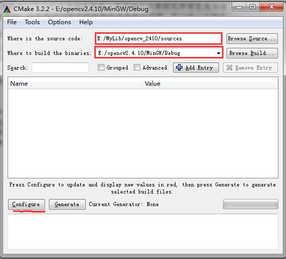
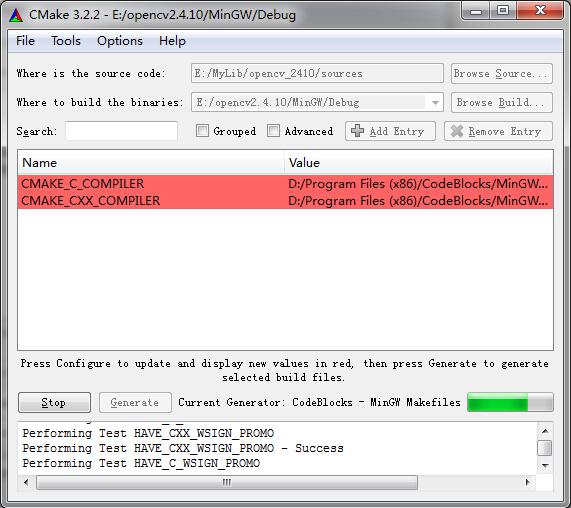
4)运行cmake，在where is the source code中填入OpenCV源代码文件的路径，比如：“…/opencv_2410/sources”；在where to build the binaries中填入编译文件需要存放的路径，比如：“…/MinGW/Debug”(存放路径文件自己定义新建一个即可)。(三点表示省略)

cmake

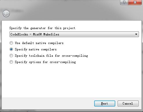
5)点击“Configure”;在Specify the generator for this project中选择MinGW Makefiles(选择刚刚安装的MinGW或者本机已有的)，选中Specify native compilers，点击“Next”。

cmake1

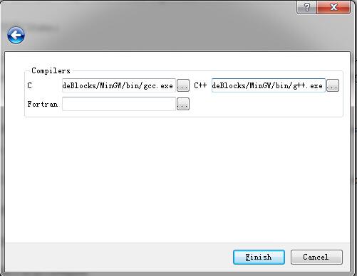
6)选择编译器路径，这里Compilers: C 选择目录为“…/MinGW/bin/gcc.exe”; C++ 选择目录为 “…/MinGw/bin/g++.exe”，点击“Finish”

cmake2

7)然后再次点“Configure”

cmake3

8)等走完进度条，选择需要的Generate选项，此处可以不操作直接点“Generate”，走完进度条便生成了“MinGW Makefiles”

cmake4

9)之后用mingw对其进行编译，cmd打开命令提示符窗口，进到刚才的保存目录，这里是“…/opencv2.4.10/MinGW/Debug”，输入“mingw32-make”，回车；等待运行完毕后，输入 mingw32-make install,回车；（此过程大约需1-2个小时）

10)运行完毕后便生成了mingw版的OpenCV库，进入“…/opencv2.4.10/MinGW/Debug/install”文件夹，便可以看到所需的头文件和库文件

cmake5

3.CodeBlocks IDE示例代码实现

我所选用的IDE是

codeblocks-13.12mingw-setup.exe

codeblocks默认使用的编译器是MinGW。

1)双击安装codeblocks

2)启动codeblocks，新建一个“Console application”项目，任意取一个名字。

3)测试代码如下

#include "cv.h"  
#include "highgui.h"  
int main()  
{  
    IplImage* img = cvLoadImage("test.jpg");  
    cvNamedWindow( "test", 0 );  
    cvShowImage("test", img);  
    cvWaitKey(0);  
    cvReleaseImage( &img );  
    cvDestroyWindow( "test" );  
    return 0;  
}

4)设置opencv相关头文件以及库文件路径

这一步是关键。因为还是有点麻烦的。

(1)右击项目名称，选build options：

codeblocks0

(2)弹出窗口，首先添加头文件路径，依次点击：Search directories->Complier->Add，选择头文件所在目录

codeblocks1

(3)选择库文件路径，依次点击Linker->Add，选择vc10下的lib库路径

codeblocks2

(4)最后点击 Linker settings，添加相应库文件，这里如果不知道自己会用到那些库文件的话，可以将vc10/lib下的所有库文件全部添加进去

codeblocks3

5)动态库调用设置

两种方法任选其一即可：

1.可以设置系统变量，将“…\opencv\build\x86\vc10\bin;”添加到系统变量中

2.将…\opencv\build\x86\vc10\bin下的所有dll文件复制到codeblocks对应工程下的bin\Debug文件夹下即可（如果会分辨opencv库文件的话，也可以只将用到的动态库复制即可）。

2022-07-24发表2016-01-12更新 yalechen 几秒读完 (大约36个字)

Welcome to yalechen's blog

This is the blog I first posted.
I will make the blog more open and share something interesting sometime.
I hope I can record my life by this way.
And
Happy New Year.God bless you.

2022-07-24发表2022-07-24更新 yalechen 18 分钟读完 (大约2728个字)

遗传算法的R语言实现

前言

遗传算法的操作使用适者生存的原则，在潜在的种群中逐次产生一个近似最优解的方案，在每一代中，根据个体在问题域中的适应度值和从自然遗传学中借鉴来的再造方法进行个体选择，产生一个新的近似解。这个过程会导致种群中个体的进化，得到的新个体比原来个体更能适应环境，就像自然界中的改造一样。

1.遗传算法原理

在遗传算法里，优化问题的解是被称为个体，它表示为一个变量序列，叫做染色体或者基因串。
编码：染色体一般被表达为简单的字符串或数字串，也有其他表示法，这一过程称为编码。
基本的过程是：

1)首先要创建种群，算法随机生成一定数量的个体，有时候也可以人工干预这个过程进行，
以提高初始种群的质量。在每一代中，每一个个体都被评价，并通过计算适应度函数得到一个适应度数值。种群中的个体被按照适应度排序，适应度高的在前面。（适应度函数）

2)产生下一代个体的种群，通过选择过程和繁殖过程完成。

选择过程，是根据新个体的适应度进行的，但同时并不意味着完全的以适应度高低作为导向，因为单纯选择适应度高的个体将可能导致算法快速收敛到局部最优解而非全局最优解，我们称之为早熟。作为折中，遗传算法依据原则：适应度越高，被选择的机会越高，而适应度低的，被选择的机会就低。初始的数据可以通过这样的选择过程组成一个相对优化的群体。

繁殖过程，表示被选择的个体进入交配过程，包括交配(crossover)和突变(mutation，交配对应算法中的交叉操作。一般的遗传算法都有一个交配概率，范围一般是0.6~1，这个交配概率反映两个被选中的个体进行交配的概率。例如，交配概率为0.8，则80%的“夫妻”个体会生育后代。每两个个体通过交配产生两个新个体，代替原来的“老”个体，而不交配的个体则保持不变。交配过程，父母的染色体相互交換，从而产生两个新的染色体，第一个个体前半段是父亲的染色体，后半段是母亲的，第二个个体则正好相反。不过这里指的半段並不是真正的一半，这个位置叫做交配点，也是随机产生的，可以是染色体的任意位置。

突变过程，表示通过突变产生新的下一代个体。一般遗传算法都有一个固定的突变常数，又称为变异概率，通常是0.1或者更小，这代表变异发生的概率。根据这个概率，新个体的染色体随机的突变，通常就是改变染色体的一个字节（0变到1，或者1变到0）。

遗传算法实现将不断的重复这个过程：每个个体被评价，计算出适应度，两个个体交配，然后突变，产生下一代，直到终止条件满足为止。一般终止条件有以下几种：

进化次数限制

计算耗费的资源限制，如计算时间、计算占用的CPU，内存等
个体已经满足最优值的条件，即最优值已经找到
当适应度已经达到饱和，继续进化不会产生适应度更好的个体
人为干预

过程：

创建初始种群
循环：产生下一代
评价种群中的个体适应度
定义选择的适应度函数
改变该种群（交配和变异）
返回第二步
满足终止条件结束

2.R语言实现

一般在进行遗传算法的时候，需要考虑的参数有：

种群规模(Population)，即种群中染色体个体的数目。
染色体的基因个数(Size)，即变量的数目。
交配概率(Crossover)，用于控制交叉计算的使用频率。交叉操作可以加快收敛，使解达到最有希望的最优解区域，因此一般取较大的交叉概率，但交叉概率太高也可能导致过早收敛。
变异概率(Mutation)，用于控制变异计算的使用频率，决定了遗传算法的局部搜索能力。
中止条件(Termination)，结束的标志。

以下是常见的R遗传算法包：

mcga包，多变量的遗传算法，用于求解多维函数的最小值。
genalg包，多变量的遗传算法，用于求解多维函数的最小值。
rgenoud包，复杂的遗传算法，将遗传算法和衍生的拟牛顿算法结合起来，可以求解复杂函数的最优化化问题。
gafit包，利用遗传算法求解一维函数的最小值。不支持R 3.1.1的版本。
GALGO包，利用遗传算法求解多维函数的最优化解。不支持R 3.1.1的版本。

那么我们今天就只针对mcga包，还有genalg包进行讲解一下吧。

1)mcga

实值优化问题。使用的变量值表示基因序列，而不是字节码，因此不需要编解码的处理。
mcga实现了遗传算法的交配和突变的操作，并且可以进行大范围和高精度的搜索空间的计算，算法的主要缺点是使用了256位的一元字母表。

install.packages("mcga")
library(mcga)

#查看mcga的定义
mcga

这是mcga的方法定义。

1 2	function (popsize, chsize, crossprob = 1, mutateprob = 0.01, elitism = 1, minval, maxval, maxiter = 10, evalFunc)

参数说明：

popsize，个体数量，即染色体数目
chsize，基因数量，限参数的数量
crossprob，交配概率，默认为1.0
mutateprob，突变概率，默认为0.01
maxiter，繁殖次数，即循环次数，默认为10
evalFunc，适应度函数，用于给个体进行评价
elitism，精英数量，直接复制到下一代的染色体数目，默认为1
minval，随机生成初始种群的下边界值
maxval，随机生成初始种群的上边界值

例子：fx=(x1-5)^2 + (x2-55)^2 +(x3-555)^2 +(x4-5555)^2 +(x5-55555)^2

# 定义适应度函数 
f <- function(x){
  #总括号
  return ((x[1]-5)^2+(x[2]-55)^2+(x[3]-555)^2+(x[4]-5555)^2+(x[5]-55555)^2)
}

# 运行遗传算法
m <- mcga(   popsize=200, 
             chsize=5, 
             minval=0.0, 
             maxval=999999, 
             maxiter=2500, 
             crossprob=1.0, 
             mutateprob=0.01, 
             evalFunc=f)

# 最优化的个体结果
print(m$population[1,])

# 执行时间
m$costs[1]

同样，当题目改为fx=(x1-5)^2 + (x2-55)^2 +(x3-555)^2 +(x4-5555)^2 +(x5-55555)^2时候：

#这是适应度函数
f<-function(x){
  return ((x[1]-7)^2 + (x[2]-77)^2 +(x[3]-777)^2 +(x[4]-7777)^2 +(x[5]-77777)^2)
}

m<-mcga(popsize=200, 
  chsize=5, 
  minval=0.0, 
  maxval=999999999.9, 
  maxiter=2500, 
  crossprob=1.0, 
  mutateprob=0.01, 
  evalFunc=f)
cat("Best chromosome:\n")
print(m$population[1,])
cat("Cost: ",m$costs[1],"\n")

2)genalg包

实现了遗传算法，还提供了遗传算法的数据可视化，给用户更直观的角度理解算法。
默认图显示的最小和平均评价值，表示遗传算法的计算进度。
直方图显出了基因选择的频率，即基因在当前个体中被选择的次数。
参数图表示评价函数和变量值，非常方便地看到评价函数和变量值的相关关系。

1 2	install.packages("genalg") library(genalg)

这是genalg函数定义：

rbga(stringMin=c(), stringMax=c(),
     suggestions=NULL,
     popSize=200, iters=100,
     mutationChance=NA,
     elitism=NA,
     monitorFunc=NULL, evalFunc=NULL,
     showSettings=FALSE, verbose=FALSE)

stringMin，设置每个基因的最小值
stringMax，设置每个基因的最大值
suggestions，建议染色体的可选列表
popSize，个体数量，即染色体数目，默认为200
iters，迭代次数，默认为100
mutationChance，突变机会，默认为1/(size+1)，它影响收敛速度和搜索空间的探测，低机率导致更快收敛，高机率增加了搜索空间的跨度。
elitism，精英数量，默认为20%，直接复制到下一代的染色体数目
monitorFunc，监控函数，每产生一代后运行
evalFunc，适应度函数，用于给个体进行评价
showSettings，打印设置，默认为false
verbose，打印算法运行日志，默认为false

例如：设fx=abs(x1-sqrt(exp(1)))+abs(x2-log(pi))，计算fx的最小值，其中x1,x2为2个不同的变量。

# 定义适应度函数
f<-function(x){
  return(abs(x[1]-sqrt(exp(1)))+abs(x[2]-log(pi)))
} 

# 定义监控函数
monitor <- function(obj){
  xlim = c(obj$stringMin[1], obj$stringMax[1]);
  ylim = c(obj$stringMin[2], obj$stringMax[2]);
  plot(obj$population, xlim=xlim, ylim=ylim, 
       xlab="pi", ylab="sqrt(50)");
}  

# 运行遗传算法 在命令行中运行
m2 = rbga(c(1,1),
           c(3,3),
           popSize=100,
           iters=1000,
           evalFunc=f,
           mutationChance=0.01,
           verbose=TRUE,
           monitorFunc=monitor
           )

#计算结果
m2$population[1,]

默认图输出，用于描述遗传过程的进展，X轴为迭代次数，Y轴评价值，评价值越接近于0越好。
在1000迭代1000次后，基本找到了精确的结果。

plot(m2)

直方图输出，用于描述对染色体的基因选择频率，即一个基因在染色体中的当前人口被选择的次数。
当x1在1.65区域时，被选择超过80次；当x2在1.146区域时，被选择超过了80次。通过直方图，我们可以理解为更优秀的基因被留给了后代。

1	plot(m2,type='hist')

参数图输出，用于描述评价函数和变量的值的相关关系。对于x1，评价值越小，变量值越准确，但相关关系不明显。对于x2，看不出相关关系。

1	plot(m2,type='vars')

以下是genalg包官方给出的例子：

# optimize two values to match pi and sqrt(50)
evaluate <- function(string=c()) {
  returnVal = NA;
  if (length(string) == 2) {
    returnVal = abs(string[1]-pi) + abs(string[2]-sqrt(50));
  } else {
    stop("Expecting a chromosome of length 2!");
  }
  returnVal
}

monitor <- function(obj) {
  # plot the population
  xlim = c(obj$stringMin[1], obj$stringMax[1]);
  ylim = c(obj$stringMin[2], obj$stringMax[2]);
  plot(obj$population, xlim=xlim, ylim=ylim, 
       xlab="pi", ylab="sqrt(50)");
}

rbga.results = rbga(c(1, 1), c(5, 10), monitorFunc=monitor, 
                    evalFunc=evaluate, verbose=TRUE, mutationChance=0.01)

plot(rbga.results)
plot(rbga.results, type="hist")
plot(rbga.results, type="vars")

2022-07-24发表2022-07-24更新 yalechen 21 分钟读完 (大约3119个字)

Java Garbage Collection Mechanism

前言

所谓“java”，其实不只是一门语言，而是一种设计的美丽，更是一种关于世界观、关于架构之美的映射。

java的底层架构，一个我所未知的世界，一个我想了解的世界。所以，我开始结识到java虚拟机(JVM)，以及java之中的垃圾收集机制。

1.JVM

既然我们时常说到”JVM(java虚拟机)”，那么所谓的java虚拟机到底是什么吗？我认为他应该是这样的：

java虚拟机，Java Virtual Machine，跟我们平常使用的Virtual PC或者VMware一样，是在操作系统上面运行的，一类模仿操作系统环境，虚构出来的计算机。Java虚拟机有自己完善的硬体架构，如处理器、堆栈、寄存器等，还具有相应的指令系统。不过，VMware等是属于系统虚拟机，而JVM是属于程序虚拟机。

既然我们都说java虚拟机十分重要，那么他为什么这么重要呢？

我们都曾弄过java的环境配置，都知道，要从Oracle官网下载jdk进行安装，知道jdk里面含有Jre，知道我们要设置计算机的环境路径。但是，对于新手来说，可能不知道，我们做这些工作，其实都是在做一件事情——配置java的虚拟机。我们所编写的java程序，经过编译之后，会生成可以在Java虚拟机上运行的字节码文件。因为每一个可以运行java程序的计算机，都拥有java虚拟机，拥有一样的运行环境。所以，在一种平台下编译生成的字节码文件，便可以在不同的平台下运行。

综上可知，JVM的优势是：屏蔽具体平台的信息，实现跨平台开发。

一般的高级语言如果要在不同的平台上运行，至少需要编译成不同的目标代码。而引入Java语言虚拟机后，Java语言在不同平台上运行时不需要重新编译。Java语言使用模式Java虚拟机屏蔽了与具体平台相关的信息，使得Java语言编译程序只需生成在Java虚拟机上运行的目标代码（字节码），就可以在多种平台上不加修改地运行。Java虚拟机在执行字节码时，把字节码解释成具体平台上的机器指令执行。

显然，没有JVM，java将不会有今天这般的辉煌。那么，JVM具体上是如何工作的呢？

JVM的工作：

1、先通过调用jdk之中的java.exe，来让操作系统装载jvm。

2、配置jvm的环境：

1）创建JVM装载环境和配置

2）装载JVM.dll

3）初始化JVM.dll并挂界到JNIENV（JNI调用接口）实例

4）调用JNIENV实例装载并处理class类

JVM在整个jdk中处于最底层的，负责操作系统的交互，用来屏蔽操作系统环境，提供一个完整的java运行环境。

首先是将JVM装入环境，JVM提供的方式是操作系统的动态链接文件。既然是装载JVM的文件，那么操作系统会在你的path下面找到你的程序的java.exe，再从里面通过各种调用寻找jvm.dll以及jvm.cfg，将其装载到操作系统，这样就可以在java中调用JVM的函数了。这些工作做完之后就开始运行java程序了。

Java程序有两种方式一种是jar包，一种是class.

运行jar,Java -jar XXX.jar运行的时候

1、Java.exe调用GetMainClassName函数，该函数先获得JNIEnv实例，然后调用Java类 Java.util.jar.JarFileJNIEnv中方法getManifest()并从返回的Manifest对象中取getAttributes(“Main-Class”)的值即jar包中文件：META-INF/MANIFEST.MF指定的Main-Class的主类名作为运行的主类。

2、之后main函数会调用Java.c中LoadClass方法装载该主类（使用JNIEnv实例的FindClass）。main函数直接调用Java.c中LoadClass方法装载该类。

如果是执行class方法。main函数直接调用Java.c中LoadClass方法装载该类。

2.Java Garbage Collection Mechanism

既然，我们已经了解到了何为“JVM”，那么我们也要接着了解一下，JVM是如何进行平时的内存分配的？

过去的语言（如C语言）要求程序员显示的分配内存、释放内存。程序在需要时分配内存，不需要时释放内存。但是这种做法常常会引起“内存泄漏”，即是说，由于某种原因是分配的内存始终没有得到释放。如果该任务不断地重复，程序最终会耗尽内存并异常终止，至少无法正常的运行下去。相比之下，java不要求程序员显式的分配内存和释放内存，避免了很多的潜在问题。java在创建对象时自动分配内存，并当该对象的引用不存在是释放这块内存。

而这也就是，java垃圾回收机制，java相对于以前的语言的优势。

java的垃圾收集机制，gc（garbage collection），是指JVM用于释放哪些不在会用的对象所占用的内存。，虽说，java语言并没有要求JVM有gc，也没有规定gc要如何进行工作，但是，常用的JVM都有GC，而且，大多数gc都使用类似的算法管理内存，和执行收集操作。

但是一般的，在java语言之中，判断一块内存空间是否符合垃圾回收器标准的标准只有两个：

给对象赋予了控制null，以后再没有调试过。
给对象赋予了新值，即重新分配了内存空间。

注：一块内存空间符合了垃圾回收器的收集标准，并不意味着这块内存控件就一定会被垃圾回收器收集。

虽说，java是自动进行内存的分配与释放的。但是，我们也可以使用System.gc()方法做到强制执行。但是，并不保证每次调用System.gc()方法就一定能够启动垃圾回收，他只不过会向jvm发出这样的一个申请，但是当地会不会真正执行垃圾回收，一切都是未知数。

所以，我们可以在执行system.gc()前，先执行finalize()方法，对对象进行强制释放内存。虽说，在没有明确释放内存志愿的情况下，java也会隐形的调用finalize()方法,终止对象，以此来释放资源。

3.Java GC

1.首先来看一下JVM内存结构，它是由堆、栈等部分组成，结构图如下所示。

JVM内存结构

1.1 堆

所有通过new创建的对象的内存都在堆中分配。显然，如果不对堆中的这些对象内存进行分类的话，是多而杂的。在不进行对象存活时间区分的情况下，每次垃圾回收都是对整个堆空间进行回收，花费时间相对会长，同时，因为每次回收都需要遍历所有存活对象，但实际上，对于生命周期长的对象而言，这种遍历是没有效果的，因为可能进行了很多次遍历，但是他们依旧存在。因此，分代垃圾回收采用分治的思想，进行代的划分，把不同生命周期的对象放在不同代上，不同代上采用最适合它的垃圾回收方式进行回收。

回收方式

年轻代:

所有新生成的对象首先都是放在年轻代的。年轻代的目标就是尽可能快速的收集掉那些生命周期短的对象。年轻代分三个区。一个Eden区，两个Survivor区(一般而言)。大部分对象在Eden区中生成。当Eden区满时，还存活的对象将被复制到Survivor区（两个中的一个），当这个Survivor区满时，此区的存活对象将被复制到另外一个Survivor区，当这个Survivor去也满了的时候，从第一个Survivor区复制过来的并且此时还存活的对象，将被复制“年老区(Tenured)”。需要注意，Survivor的两个区是对称的，没先后关系，所以同一个区中可能同时存在从Eden复制过来对象，和从前一个Survivor复制过来的对象，而复制到年老区的只有从第一个Survivor去过来的对象。而且，Survivor区总有一个是空的。同时，根据程序需要，Survivor区是可以配置为多个的（多于两个），这样可以增加对象在年轻代中的存在时间，减少被放到年老代的可能。

年老代:

在年轻代中经历了N次垃圾回收后仍然存活的对象，就会被放到年老代中。因此，可以认为年老代中存放的都是一些生命周期较长的对象。

持久代:

用于存放静态文件，如今Java类、方法等。持久代对垃圾回收没有显著影响，但是有些应用可能动态生成或者调用一些class，例如Hibernate等，在这种时候需要设置一个比较大的持久代空间来存放这些运行过程中新增的类。持久代大小通过-XX:MaxPermSize=进行设置。

1.2 栈

每个线程执行每个方法的时候都会在栈中申请一个栈帧，每个栈帧包括局部变量区和操作数栈，用于存放此次方法调用过程中的临时变量、参数和中间结果。

2.VM垃圾回收机制

针对上述的分类，GC有两种类型：Scavenge GC和Full GC。

2.1 Scavenge GC

一般情况下，当新对象生成，并且在Eden申请空间失败时，就会触发Scavenge GC，对Eden区域进行GC，清除非存活对象，并且把尚且存活的对象移动到Survivor区。然后整理Survivor的两个区。这种方式的GC是对年轻代的Eden区进行，不会影响到年老代。因为大部分对象都是从Eden区开始的，同时Eden区不会分配的很大，所以Eden区的GC会频繁进行。因而，一般在这里需要使用速度快、效率高的算法，使Eden去能尽快空闲出来。

2.2 Full GC

对整个堆进行整理，包括Young、Tenured和Perm。因为需要对整个块进行回收，所以比Scavenge GC要慢，因此应该尽可能减少Full GC的次数。在对JVM调优的过程中，很大一部分工作就是对于FullGC的调节。有如下原因可能导致Full GC：

年老代（Tenured）被写满
持久代（Perm）被写满
System.gc()被显示调用
上一次GC之后Heap的各域分配策略动态变化

下次跟大家，分享一下，垃圾回收机制的几个算法问题吧。

2022-07-24发表2022-07-24更新 yalechen 9 分钟读完 (大约1292个字)

RoboCup Rescue 2015 – Rescue Simulation League Team Description S.O.S (Iran)

前言

这是我过去一年一直在准备并参与的一个比赛RoboCup Recuse Similation League。虽然现在比赛已经结束，但还是抽出时间整理了下以前的东西。为了下届学弟学妹们，也翻译了些许文章。而这一片是描述我们在世界级别比赛上的最大的对手，世界冠军S.O.S。这是原文链接。以下便开始翻译内容。

摘要：

SOS团队是众所周知的，在救援仿真联赛中表现出色。我们已经在这个比赛中取得了很多的奖项。去年，我们在巴西举行的机器人世界杯获得第一名。我们团队已经发展了多年，主要是老成员，这些年在不同的比赛中我们的基本代码的得分非常稳定，本文旨在提高老战略和解决新出现的逻辑错误和增加新的功能。

1.介绍

该S.O.S.基础AT的能力和技能，在往年的TDP（2010- 2014年）进行了说明，因此本文所要描绘的是我们的计划，就2015年机器人世界杯新战略的细节改进进行介绍。

去年SOS成员开发全速和低速通信，但到2015年机器人世界杯大赛SOS的主要重点是没有沟通的地图，这种方式专门为消防官兵和警察部队AT创造。在自然灾害中所有类型的事件会发生。正因为如此，在最困难的情况下，我们将执行这么多的活动，来操纵我们的代码。

2 agent

2.1 警察

我们去年的TDP没有讨论被添加到Policeforce代码的新功能。因此，在今年的TDP，我们注重描写警察的算法和方法。

2.1.1 清理系统

改变在2013年模拟服务器中大量的AT卡在地图上的陡峭的边缘问题。定义此问题时必须指出的是，当AT是停留在一个凹区域，其他代理将包围它并引起排斥力卡ＡＴ。其结果是，大量的时间将在释放该ＡＴ的过程中被浪费。

清理时与街道不具有相同的方向原因。道路有在关节角的方向之间的陡峭的角度，这将导致在凹形区域中的间隙的棱角产生影响。简单和基本的解决办法是清除整条道路，但我们已经避免了，因为这会浪费大量的周期。
　
该SOS警方已经设计和开发新的系统和算法，将减小卡在边缘AT的概率。清除时，我们的算法考虑到所有的未来路径，然后选择最佳路径（基于接下来的步骤），同时考虑所有选项（而不是选择和清除的道路的主要方向），这将导致降低卡在陡峭的边缘可能性。图（1）图（2），我们可以比较SOS新的结算方法，由浙江大学队结算。

SOS

2.1.2 消防队到达火区

一个在警察部队的其他变动是增加了中断状态，用于帮助消防队处理火灾。如果一个警察看到或感知火灾发生后，AT开始估计火灾的大小。如果猜测，火灾是相当小的尺寸，警方会放弃自己的任务，首先释放消防大队AT和火之间的路径，所以大火将更快熄灭。

2.1.3 检查火灾的概率状态

加入警队的另一个特点是检查火灾概率状态。在这种状态下，如果警方检测一些建筑物的高温，AT开始估计火灾可能发生。如果发生火灾的地区是ＡＴ附近，ＡＴ将清除道路，所以可以阻止火灾发生。

2.1.4　无通讯世界模型

我们的警察部队也更新与消防队的通讯，这是在没有通信战略的世界模型下。在没有沟通的策略下，如果ＡＴ检测火的集群，遵循火找到它的边界。但是，什么是比找到火并通知火的新信息消防大队代理更重要。警方代理发现消防大队的负责灭火，并更新了消防的信息。由于没有沟通，根据他们的旧世界模式不明，为消防队的最有可能的地方，警方搜查了代理商的确切位置。然后警察代理更新世界模型的每个消防队的信息，如果火剂的最后一次更新的时间超过15个周期。

2022-07-24发表2022-07-24更新 yalechen 10 分钟读完 (大约1425个字)

Ambition

野心，你有想要颠覆这个星球的野心吗？

有点中二，有点热血，一句话可以点燃撩在心头的蠢动。原本有点玩笑意味的话，却是一些人一生的信条。这就是我在钢总和刀哥身上看到的。

前几天，有幸能够听到原WPS技术副总裁、现中科云华CEO杨钢钢总，以及原阿里金融CTO、小米金融总经理、现福米信息CEO王安全刀哥的分享，能够跟他们坐一起畅聊。这是一次难得的机会，倾听互联网业界前辈的见解，得窥行业秘辛。

钢总是个酷劲十足而又不失风趣的技术达人兼霸道总裁。有句话叫做，无形装逼最为致命。用在钢总身上最为贴切，境界确实不一样。钢总技术出身，在WPS呆了十年，公司里面一有难题就会找他，实力过硬。按他的说法就是，大大小小技术领域都玩过了。后来在金山跟雷军聊创业理念后，他决定出来创业，也就有了今天的中科云华。不过我比较感兴趣的是，他在金山时跟雷军、傅盛叫板时候的不羁与洒脱。这要是我的话，可能话都说不利索。

刀哥是个很沉稳的人，说话慢条斯理、逻辑清晰，不愧技术出身又成功转型为生意人。关于金融，刀哥有着自己的一套见解，认为未来的金融应该是一个标准化的市场，标准化交易。关于学习能力，刀哥认识是，一种能够在短时间内迅速掌理清新领域主要框架的能力。刀哥还给我们讲了他的年少轻狂，大学未毕业就带着基友跑到上海出来创业。当然这也不是主要的。那晚最让我记忆犹新的一句话是，刀哥拒绝雷军的挽留时讲的，“我要当的是老大，你给不了我”。

我曾经想过一个问题，怎样的人会在无形中让别人信服？

现在我想给出一个答案，野心。这是我从身边有所成的人身上可以看到的。追求技术巅峰的野心，想要扬名立万的野心，想要建立起一个商业帝国的野心，想要改变生活的野心，乃至于要颠覆这个星球的野心。目标驱动主义，不达目标不罢休，不到棺材不落泪，甚至是置之死地而后生。突破现有的自己，想要紧紧握住通往梦想的门票。这就是野心。而这也是很难在一个大学生身上看到的，难能可贵的。

作为大学生，我很难能够从身边同学的眼中看到渴望，看到野心，更多的反而是一种萎靡，通宵打LOL的疲倦，无所事事的宅，无所适从的迷茫。时光，在他们身上变成了荒土。每一个能够进入大学的学生，都曾经是不一般的人，都怀着梦想踏进校门的。但是大学没有给到他们想要的，没有教给他们独立的能力，前瞻的眼光，明确的目标，深刻的野心，反而丢弃了用十几年义务教育才养成的学习能力。

肖老师说过，做科研只能是那些懂得精神满足的人才能做成功，比如一生都在say no的佩雷尔曼。因为只有在精神满足的情况下，你才能够全神贯注的进入到科研的领域中去。而对于野心，我认为正好相反，只有那些饥渴的人才能够拥有，因为精神上的饥渴，让他们极其渴望拥有，并且无从选择的去拥有，这就是野心。而这也是常人罕见的体验，常人只会甘于满足，认为，自讨苦吃的，不值得。没有人甘于平庸，但是，以大多数人努力的程度，注定平庸。

已经大三下，对于这几年的大学生涯，虽有遗憾，但却是实实在在的充实，我感谢自己的努力。但是，平常的忙里忙外，却鲜少有所成就，甚至有时候都是在瞎忙，回首也不知道自己在忙些什么。或许，说白了，自己确实是没有野心，没有极其渴望得到某样东西的欲望，随遇则安，得过且过。这不行，得治。

往者不可谏，来者犹可追。过去难以改变，也不需要改变，那就去改变未来吧。我不知道自己有一天会不会有颠覆世界的野心，也不知道自己能不能够改变这个世界。我只希望在我的每一个人生阶段，都能够有一个不一般的目标，一个小野心，跳出身边的圈子，找到更大的世界。

2022-07-24发表2022-07-24更新 yalechen 11 分钟读完 (大约1688个字)

No Compromise

昨天又是翘了一节课，而这次翘课又与往常稍微不一样，因为这是翘了中南的课，却到了湖大的课堂听讲。有时候觉得蛮有趣的，因为这是交了一份大学学费，上了两所大学。

昨天的课叫做，这个校友有点6，官方名字是“熊晓鸽奖学金、奖教金、我最敬爱的老师”颁奖仪式。

我跟几个同学早早来到了会场，坐到了前排。我是认真听完了全程，并随着掌声不自禁的喝彩，仿佛自身便是一名湖大人，能够感受到湖大的激情以及熊晓鸽熊先生的感召力之强。

全程中，有几个人我是格外印象深刻。一个是那位头发花白但面容依旧俊朗的主持人老师。开始是因为他充满磁性的嗓音以及沉稳的主持风格，后来是对于他在台下认真仔细准备主持词时候的敬佩。他身着中山装，身上还有着老一辈人的沉稳执着。

第二个是湖大的新任校长段校长。这个关注他的点就是，纯粹的，他能够听得到湖大学生的心声，保证不会断网断电，能够提前对来场嘉宾做好功课，以及能够抓住一切能够与学生交流的机会上台解答学生的问题。是个好校长。

最后一个当然就是主角熊晓鸽了。在昨天之前我也是不了解熊晓鸽是为何人物。于是专门去收集了下他的履历。然后，就只剩下跪舔了。

熊先生现任IDG（美国国际数据集团）全球常务副总裁兼亚洲区总裁，是IDG资本创始合伙人，被誉为中国引入高科技产业风险基金的第一人，曾投资过百度、腾讯、携程、当当、搜狐、哔哩哔哩等等四百多家公司，一个人掌握着10亿投资资金。然而熊先生却也是平困出身，年少是当过电工，后考上湖大，开始求学生涯，在湖大读书期间最喜欢的是晚上跑到岳麓山上思考。在新华社实习时候，梦想新华社外派战地记者。获得恩师推荐，来到波士顿大学，只用了八个月夺得新闻传播学院硕士学位。接着进入塔夫茨大学弗莱彻法律与外交学院攻读国际经济与商理博士学位。

台上的熊先生，没有所谓的威严，比较亲和，比较风趣，而且比较坑队友。因为正值移动互联网岳麓峰会，于是他邀请了湖湘会的朋友过来，包括58公司董事长姚劲波、拓维信息集团总裁李宇新等等。然后，然后就是一堆段子手的主场了，期间不乏掌声雷动。熊先生真是热爱着他的母校，就那一会，湖大就又有了至少一千多万的捐款，而且把这个熊晓鸽奖学金的含金量蹭蹭的给往上提高了许多，各位大佬都给予了应允。

这次课切切实实的给我证明了名校的价值所在——名校资源。这个资源不仅仅是说，你在学校课程上的教学资源，而是你整个职业生涯里面的社会资源。每一个校园都是一个圈子，维系这个圈子的是情怀、校友情怀，圈子里面的人相互关照，圈子外的人很难介入，比如耶鲁大学的骷髅会。所以，在学校里面是，有着满满的机会的。另外，名校与职工技校的区别在于，他不是技能培训机构，他培养的是思维，更是一种与世界平齐的视界，因为你面对的都是来自各个领域顶端的人物。可惜，国内高校并没有把这方面做的很好。

更加可惜的是，作为学生，还处于职业生涯的规划状态，缘由怯懦，总是对这些机会视若无睹。每当遇到这样的讲座，学校都只能是强制地让几个班的同学去充当水军了，因为学生对于这些所谓的大佬成功人士，是没有概念的，认为是与自己遥不可及的，觉得自己还是个学生，还是个孩子，还不需要考虑这些事情，他们是谁管我鸟事。校园的象牙塔里面，他们是安逸的，还没有意识到没个几年就要毕业，即将要面对这些柴米油盐酱醋茶。毕业不可怕，迷茫不可怕，选择也不可怕，可怕的是，在不知不觉之间，变得别无选择，在迷迷糊糊的时候，做出了最坏的选择而不自知，最后只能将就。

这几年，我也是常常做项目，也跟着别人到处跑，自己越来越清楚的感受到，技术不是生活的全部。人与计算机打交道，说到底还是简单直接的，因为计算机是不会欺骗，他对你是永远正直的。而人与人之间的门道，却是不可捉摸的，没有原理可言，没有所谓的定律可以依据。在计算机的01之间，或许程序员便是上帝，但是在这个社会框架里面，站在顶端主导世界变革的却永远不会是一个只知道01的人。所以，一直认为无形中便能够让人信服的人十分令人敬佩。

看着台上刚从美国波士顿飞回来的学姐，讲着她对晓鸽学长知遇之情的感激，我开着玩笑对旁边的同学说，“过不了十年，站在上面讲的人的就是你了”。他说好。

这是一篇反思文，凑合着看吧。